Basic Usage Tutorial

cellpin imputes the missing genes of spatially-resolved cells by leveraging a single-cell RNA reference data.
This notebook walks through three complete workflows:

Section	Description
A — Standard	Train on all overlapping genes and impute the full reference gene space
B — Held-out evaluation	Hold out panel genes before training to benchmark imputation accuracy

Before running: update the file paths in Load data cell to point to your own .h5ad files.

Setup

import cellpin
import torch
import scanpy as sc
import numpy as np
import yaml
from pathlib import Path
from time import time

Helper functions

Two evaluation helpers used throughout the notebook:

• correlation_panel — mean Pearson correlation between observed and imputed counts for the training panel genes

• correlation_heldout — same metric, but restricted to genes that were held out during training (Option B only)

def correlation_panel(adata_imputed, layer_real, layer_imputed):
    """Mean per-gene Pearson r between two layers. Genes with -2 sentinel are excluded."""
    counts_mat = adata_imputed.layers[layer_real]
    imputed_mat = adata_imputed.layers[layer_imputed]
    if hasattr(counts_mat, "toarray"):
        counts_mat = counts_mat.toarray()
    if hasattr(imputed_mat, "toarray"):
        imputed_mat = imputed_mat.toarray()

    valid_idx = np.where(~(counts_mat == -2).any(axis=0))[0]
    pearsons = []
    for j in valid_idx:
        x, y = counts_mat[:, j], imputed_mat[:, j]
        if np.std(x) > 0 and np.std(y) > 0:
            pearsons.append(np.corrcoef(x, y)[0, 1])
        else:
            pearsons.append(np.nan)

    mean_r = np.nanmean(pearsons)
    print(f"Valid genes (no sentinel): {len(valid_idx)}")
    print(f"Mean Pearson r           : {mean_r:.4f}")


def correlation_heldout(adata_imputed, sp_adata_full, heldout_genes, layer_real="counts", layer_imputed="imputed"):
    """Evaluate imputation accuracy on genes held out during training."""
    assert sp_adata_full.n_obs == adata_imputed.n_obs, "Cell count mismatch between sp_adata_full and adata_imputed."

    pearsons = []
    for gene in heldout_genes:
        if gene not in sp_adata_full.var_names or gene not in adata_imputed.var_names:
            print(f"  [{gene}] not found — skipping")
            continue
        real = sp_adata_full[:, gene].layers[layer_real].toarray().flatten().astype(float)
        imputed = adata_imputed[:, gene].layers[layer_imputed].toarray().flatten().astype(float)
        if np.std(real) == 0 or np.std(imputed) == 0:
            print(f"  [{gene}] zero variance — skipping")
            continue
        r = np.corrcoef(real, imputed)[0, 1]
        pearsons.append(r)
        print(f"  {gene:20s}  Pearson = {r:.4f}")

    mean_r = np.nanmean(pearsons)
    print(f"\nMean Pearson over {len(pearsons)} held-out genes: {mean_r:.4f}")

---

A) Standard Workflow — Full Panel

The standard cellpin workflow in four steps:

1. Load a single-cell reference (sc_adata) and a spatial dataset (sp_adata)

2. Run cellpin.pp.setup_data() to align gene spaces

3. Train a CellPin model on the scRNA reference

4. Impute the full gene space for every spatial cell

All overlapping genes between the two datasets are used as panel input.

A.1 — Load data

Both objects need raw integer counts — either in .X or in a named layer (set LAYER accordingly).

• sc_adata: single-cell reference atlas (full / highly-variable gene space)

• sp_adata: spatially-resolved dataset (panel genes only)

Example data

• Source dataset: 10x Genomics Xenium breast preview dataset

• First described in: Nature Communications (2023)

• Processing: data were processed according to standard single-cell best practices

• scRNA preprocessing: subset to Xenium panel genes plus 1,000 additional highly variable genes

• Spatial data: subsampled, with a normalized layer added

• Samples used:

  • Spatial: In Situ Sample 1, Replicate 1

  • Single-cell: FRP

LAYER = "counts"  # layer key with raw integer counts; set to None to use .X

sc_adata = cellpin.pp.load_sc_example()
sp_adata = cellpin.pp.load_sp_example()

print(f"sc_adata : {sc_adata.n_obs:,} cells × {sc_adata.n_vars:,} genes")
print(f"sp_adata : {sp_adata.n_obs:,} cells × {sp_adata.n_vars:,} spatial genes")

sc_adata : 23,867 cells × 1,307 genes
sp_adata : 30,600 cells × 313 spatial genes

A.2 — Gene alignment check

Confirm which spatial genes are present in the scRNA reference before calling setup_data().
Any missing genes will be dropped automatically, but it is good to know upfront.

sc_genes = sc_adata.var_names
sp_genes = sp_adata.var_names

missing = sp_genes.difference(sc_genes)
if len(missing) == 0:
    print(f"All {len(sp_genes)} spatial genes are present in sc_adata ✓")
else:
    print(f"WARNING: {len(missing)} spatial gene(s) not in sc_adata (will be dropped by setup):")
    print(sorted(missing))

overlap = sp_genes.intersection(sc_genes)
print(f"\nPanel size (overlap)        : {len(overlap)} genes")
print(f"scRNA-only genes (to impute): {len(sc_genes) - len(overlap)} genes")

WARNING: 6 spatial gene(s) not in sc_adata (will be dropped by setup):
['AKR1C1', 'ANGPT2', 'BTNL9', 'CD8B', 'POLR2J3', 'TPSAB1']

Panel size (overlap)        : 307 genes
scRNA-only genes (to impute): 1000 genes

A.3 — Setup and train

sc_dataset, sp_dataset = cellpin.pp.setup_data(
    sc_adata, sp_adata, layer=LAYER
)  # add batch_key="batch" if needed -recommended for reference atlases

============================================================
[cellpin.pp.setup] Setting up CellPin datasets
============================================================
[cellpin.pp.setup] sc_adata :   23,867 cells  ×    1,307 genes
[cellpin.pp.setup] st_adata :   30,600 cells  ×      313 spatial genes
[cellpin.pp.setup] Expression read from layer='counts'
[cellpin.pp.setup] WARNING: 6 spatial gene(s) not found in sc_adata — will be dropped:
  ['AKR1C1', 'ANGPT2', 'BTNL9', 'CD8B', 'POLR2J3', 'TPSAB1']
[cellpin.pp.setup] Panel    : 307 genes overlap (98.1% of spatial genes retained)
[cellpin.pp.setup] Imputed  : 1,307 genes total in sc space (1,000 genes to impute, not in panel)
[cellpin.pp.setup] sc_dataset: 23,867 cells, 1,307 genes total, 307 panel genes
[cellpin.pp.setup] st_dataset: 30,600 cells, 307 panel genes

time_start = time()
model_A = cellpin.CellPin(sc_dataset)
model_A.fit(
    sc_dataset, pretrain_epochs=50, train_epochs=60, save_checkpoints=False
)  # save_checkpoints=True is much slower and not needed for this tutorial
print(f"Training time: {(time() - time_start) / 60:.2f} minutes")

Epoch 49: 100%|██████████| 75/75 [00:02<00:00, 25.20it/s, v_num=0, val_loss=457.0, val_reconst_loss=438.0, val_kl_loss=16.60, val_kl_l_loss=2.350, val_pearson_loss=0.484, train_loss=465.0, train_reconst_loss=445.0, train_kl_loss=17.40, train_kl_l_loss=2.390, train_pearson_loss=0.464]   
Epoch 58: 100%|██████████| 75/75 [00:03<00:00, 20.83it/s, v_num=0, val_loss=524.0, val_reconst_loss=438.0, val_kl_loss=55.80, val_kl_l_loss=2.490, val_distill_loss=0.0722, val_snn_loss=1.630, val_inv_loss=0.210, val_snn_temperature=0.104, val_pearson_loss=0.468, train_loss=520.0, train_reconst_loss=435.0, train_kl_loss=59.30, train_kl_l_loss=2.510, train_distill_loss=0.0816, train_snn_loss=1.670, train_inv_loss=0.223, train_snn_temperature=0.104, train_pearson_loss=0.436]
Training time: 6.10 minutes

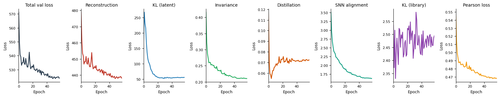
model_A.pl.losses(smooth=5)

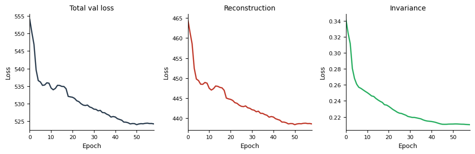
model_A.pl.losses(keys="all")

A.4 — Impute

return_norm=True adds an area-normalised log1p layer (imputed_norm).
Set area_key=None if your spatial data has no cell_area column.

time_start = time()
dl_A = torch.utils.data.DataLoader(sp_dataset, batch_size=512, shuffle=False)

adata_imputed_A = model_A.impute(
    dl_A,
    obs_adata=sp_adata,
    return_norm=True,
    area_key="cell_area",
    nb_count_samples=20,
    #return_int=True is recomended for denoising data and performing downstream analyses
)
print(f"Imputation time: {(time() - time_start) / 60:.2f} minutes")
print(adata_imputed_A)

Embedding and imputing cells (MC, 50 samples)...
[CellPin.impute] Panel gene order confirmed ✓
  [impute] Filling 1000 gene(s) absent from obs_adata layers with sentinel -2.0
  [impute] Filling 1000 gene(s) absent from obs_adata layers with sentinel -2.0
Imputation time: 1.15 minutes
AnnData object with n_obs × n_vars = 30600 × 1307
    obs: 'cell_id', 'transcript_counts', 'control_probe_counts', 'control_codeword_counts', 'total_counts', 'cell_area', 'nucleus_area', 'region'
    obsm: 'X_cellpin', 'spatial'
    layers: 'counts', 'log1p_norm', 'imputed', 'imputed_norm'

A.5 — Evaluate

Pearson correlation between observed and imputed counts for panel genes.

print("=== Count space ===")
correlation_panel(adata_imputed_A, layer_real="counts", layer_imputed="imputed")

print("\n=== Log-normalised space ===")
correlation_panel(adata_imputed_A, layer_real="log1p_norm", layer_imputed="imputed_norm")

=== Count space ===
Valid genes (no sentinel): 307
Mean Pearson r           : 0.5938

=== Log-normalised space ===
Valid genes (no sentinel): 307
Mean Pearson r           : 0.4980

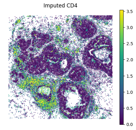
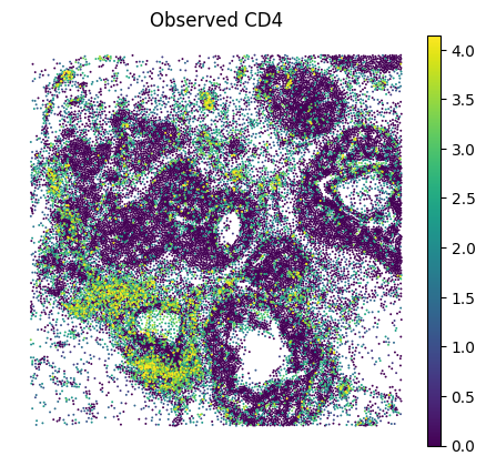
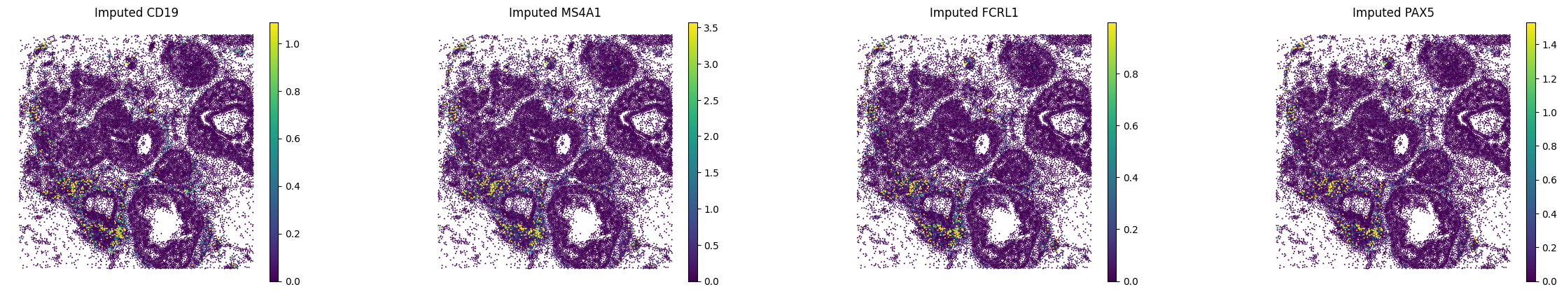
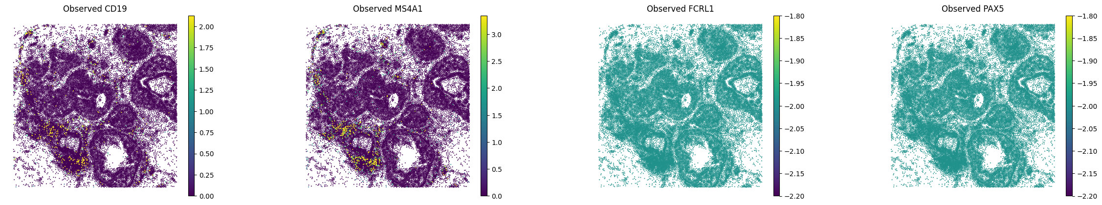
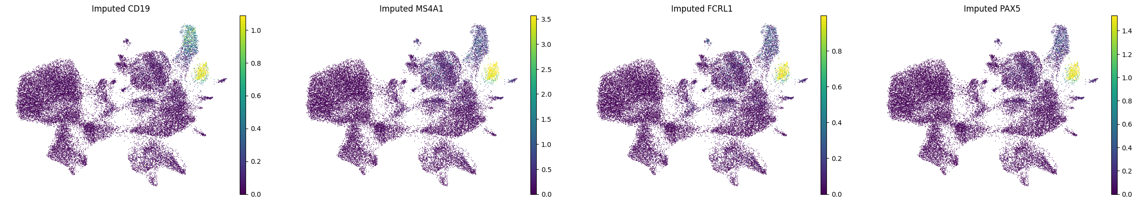
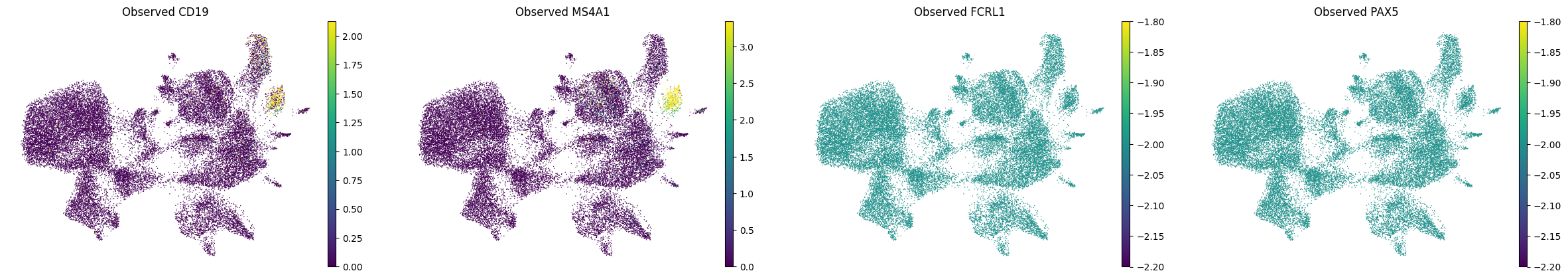
A.6 — Visualise

Spatial maps and UMAP for a few marker genes.
MS4A1 and CD19 were in the panel; FCRL1 and PAX5 are purely imputed. (All B cell genes, expected to co-localise)

GENE = "CD4"  # edit as needed

sc.pl.spatial(
    adata_imputed_A, layer="imputed_norm", color=GENE, spot_size=15, vmax="p99", frameon=False, title=f"Imputed {GENE}"
)
sc.pl.spatial(
    adata_imputed_A, layer="log1p_norm", color=GENE, spot_size=15, vmax="p99", frameon=False, title=f"Observed {GENE}"
)

bcells = ["CD19", "MS4A1", "FCRL1", "PAX5"]

print("Spatial plots — B-cell markers:")
sc.pl.spatial(
    adata_imputed_A,
    layer="imputed_norm",
    color=bcells,
    spot_size=15,
    vmax="p99",
    frameon=False,
    title=[f"Imputed {g}" for g in bcells],
)
sc.pl.spatial(
    adata_imputed_A,
    layer="log1p_norm",
    color=bcells,
    spot_size=15,
    vmax="p99",
    frameon=False,
    title=[f"Observed {g}" for g in bcells],
)

Spatial plots — B-cell markers:

A.7 — UMAP from cellpin embeddings

Cell embeddings in obsm["X_cellpin"] can be used directly to build a neighborhood graph and compute a UMAP

sc.pp.neighbors(adata_imputed_A, use_rep="X_cellpin")
sc.tl.umap(adata_imputed_A)

print("UMAP — B-cell markers:")
sc.pl.umap(adata_imputed_A, color=bcells, layer="imputed_norm", vmax="p99", title=[f"Imputed {g}" for g in bcells],frameon=False)
sc.pl.umap(adata_imputed_A, color=bcells, layer="log1p_norm", vmax="p99", title=[f"Observed {g}" for g in bcells],frameon=False)

UMAP — B-cell markers:

---

B) Held-Out Gene Evaluation

To benchmark how well cellpin imputes genes it has never seen during training, we:

1. Randomly sample a fraction of panel genes as held-out genes

2. Remove them from the spatial input before setup_data()

3. Train and impute as normal

4. Compare imputed values against the ground-truth counts for those held-out genes

The held-out Pearson correlation is the most honest imputation benchmark.

B.1 — Define held-out genes

rng = np.random.default_rng(42)

# Panel genes in sc_adata order — consistent with setup_data()'s internal ordering
panel_genes_all = [g for g in sc_adata.var_names if g in set(sp_adata.var_names)]
print(f"Full panel size: {len(panel_genes_all)} genes")

HOLDOUT_FRACTION = 0.10  # hold out 10 % of the panel
n_holdout = max(1, int(len(panel_genes_all) * HOLDOUT_FRACTION))
heldout_genes = rng.choice(panel_genes_all, size=n_holdout, replace=False).tolist()
training_genes = [g for g in panel_genes_all if g not in heldout_genes]

print(f"Held-out genes : {n_holdout}  → {heldout_genes[:5]} ...")
print(f"Training panel : {len(training_genes)} genes")

Full panel size: 307 genes
Held-out genes : 30  → ['NDUFA4L2', 'CCDC6', 'LEP', 'CCL8', 'ELF3'] ...
Training panel : 277 genes

# Build the reduced spatial object (held-out genes removed)
sp_adata_reduced = sp_adata[:, training_genes].copy()

assert len(set(heldout_genes) & set(sp_adata_reduced.var_names)) == 0, (
    "Held-out genes still present in reduced sp_adata!"
)
print(
    f"sp_adata_reduced: {sp_adata_reduced.n_obs:,} cells × {sp_adata_reduced.n_vars:,} genes (held-out genes removed ✓)"
)

sp_adata_reduced: 30,600 cells × 277 genes (held-out genes removed ✓)

B.2 — Setup and train

sc_dataset_B, sp_dataset_B = cellpin.pp.setup_data(sc_adata, sp_adata_reduced, layer=LAYER)

============================================================
[cellpin.pp.setup] Setting up CellPin datasets
============================================================
[cellpin.pp.setup] sc_adata :   23,867 cells  ×    1,307 genes
[cellpin.pp.setup] st_adata :   30,600 cells  ×      277 spatial genes
[cellpin.pp.setup] Expression read from layer='counts'
[cellpin.pp.setup] Panel    : 277 genes overlap (100.0% of spatial genes retained)
[cellpin.pp.setup] Imputed  : 1,307 genes total in sc space (1,030 genes to impute, not in panel)
[cellpin.pp.setup] sc_dataset: 23,867 cells, 1,307 genes total, 277 panel genes
[cellpin.pp.setup] st_dataset: 30,600 cells, 277 panel genes

model_B = cellpin.CellPin(sc_dataset_B)
model_B.fit(
    sc_dataset_B, pretrain_epochs=50, train_epochs=60, save_checkpoints=False
)  # save_checkpoints=True is much slower and not needed for this tutorial

Epoch 0:  39%|███▊      | 29/75 [00:01<00:01, 25.61it/s, v_num=1]
Epoch 49: 100%|██████████| 75/75 [00:03<00:00, 23.22it/s, v_num=1, val_loss=456.0, val_reconst_loss=436.0, val_kl_loss=17.00, val_kl_l_loss=2.390, val_pearson_loss=0.483, train_loss=464.0, train_reconst_loss=444.0, train_kl_loss=17.70, train_kl_l_loss=2.380, train_pearson_loss=0.465] 
Epoch 59: 100%|██████████| 75/75 [00:03<00:00, 19.93it/s, v_num=1, val_loss=521.0, val_reconst_loss=436.0, val_kl_loss=55.60, val_kl_l_loss=2.470, val_distill_loss=0.0726, val_snn_loss=1.660, val_inv_loss=0.214, val_snn_temperature=0.104, val_pearson_loss=0.470, train_loss=522.0, train_reconst_loss=436.0, train_kl_loss=59.50, train_kl_l_loss=2.520, train_distill_loss=0.0836, train_snn_loss=1.730, train_inv_loss=0.231, train_snn_temperature=0.104, train_pearson_loss=0.440]

B.3 — Impute

dl_B = torch.utils.data.DataLoader(sp_dataset_B, batch_size=512, shuffle=False)

adata_imputed_B = model_B.impute(
    dl_B,
    obs_adata=sp_adata_reduced,
    return_norm=True,
    area_key="cell_area",
    nb_count_samples=20,
    #return_int=True is recomended for denoising data and performing downstream analyses
)
print(adata_imputed_B)

Embedding and imputing cells (MC, 50 samples)...
[CellPin.impute] Panel gene order confirmed ✓
  [impute] Filling 1030 gene(s) absent from obs_adata layers with sentinel -2.0
  [impute] Filling 1030 gene(s) absent from obs_adata layers with sentinel -2.0
AnnData object with n_obs × n_vars = 30600 × 1307
    obs: 'cell_id', 'transcript_counts', 'control_probe_counts', 'control_codeword_counts', 'total_counts', 'cell_area', 'nucleus_area', 'region'
    obsm: 'X_cellpin', 'spatial'
    layers: 'counts', 'log1p_norm', 'imputed', 'imputed_norm'

B.4 — Evaluate

Two metrics:

• Panel Pearson — reconstruction quality on the training genes (sanity check)

• Held-out Pearson — true imputation benchmark on genes the model never saw

print("=== Training panel genes (count space) ===")
correlation_panel(adata_imputed_B, layer_real="counts", layer_imputed="imputed")

=== Training panel genes (count space) ===
Valid genes (no sentinel): 277
Mean Pearson r           : 0.5963

print("=== Held-out genes — count space ===")
correlation_heldout(
    adata_imputed_B,
    sp_adata_full=sp_adata,  # sp_adata (full) has ground-truth counts for held-out genes
    heldout_genes=heldout_genes,
    layer_real="counts",
    layer_imputed="imputed",
)

=== Held-out genes — count space ===
  NDUFA4L2              Pearson = 0.1975
  CCDC6                 Pearson = 0.6173
  LEP                   Pearson = 0.3429
  CCL8                  Pearson = 0.1985
  ELF3                  Pearson = 0.6551
  ENAH                  Pearson = 0.4506
  TIMP4                 Pearson = 0.2919
  KRT14                 Pearson = 0.8070
  ITGAX                 Pearson = 0.7537
  LYZ                   Pearson = 0.7676
  GNLY                  Pearson = 0.5750
  CX3CR1                Pearson = 0.4900
  SPIB                  Pearson = 0.3898
  CXCL12                Pearson = 0.8441
  KRT23                 Pearson = 0.8277
  DNAAF1                Pearson = 0.0584
  AGR3                  Pearson = 0.6253
  FOXA1                 Pearson = 0.8592
  FOXP3                 Pearson = 0.3508
  PTN                   Pearson = 0.7818
  PDCD1LG2              Pearson = 0.2287
  CCND1                 Pearson = 0.7912
  SQLE                  Pearson = 0.4533
  ANKRD30A              Pearson = 0.8562
  SERPINA3              Pearson = 0.7612
  CEACAM8               Pearson = -0.0366
  GPR183                Pearson = 0.5304
  CLECL1                Pearson = 0.2589
  LILRA4                Pearson = 0.7407
  CCPG1                 Pearson = 0.4594

Mean Pearson over 30 held-out genes: 0.5309

print("=== Held-out genes — log-normalised space ===")
correlation_heldout(
    adata_imputed_B,
    sp_adata_full=sp_adata,
    heldout_genes=heldout_genes,
    layer_real="log1p_norm",
    layer_imputed="imputed_norm",
)

=== Held-out genes — log-normalised space ===
  NDUFA4L2              Pearson = 0.1717
  CCDC6                 Pearson = 0.5261
  LEP                   Pearson = 0.1451
  CCL8                  Pearson = 0.1529
  ELF3                  Pearson = 0.6506
  ENAH                  Pearson = 0.3184
  TIMP4                 Pearson = 0.0974
  KRT14                 Pearson = 0.7578
  ITGAX                 Pearson = 0.5899
  LYZ                   Pearson = 0.6539
  GNLY                  Pearson = 0.3986
  CX3CR1                Pearson = 0.4187
  SPIB                  Pearson = 0.3675
  CXCL12                Pearson = 0.7626
  KRT23                 Pearson = 0.7281
  DNAAF1                Pearson = 0.0097
  AGR3                  Pearson = 0.5790
  FOXA1                 Pearson = 0.8434
  FOXP3                 Pearson = 0.3118
  PTN                   Pearson = 0.7032
  PDCD1LG2              Pearson = 0.1542
  CCND1                 Pearson = 0.6785
  SQLE                  Pearson = 0.3021
  ANKRD30A              Pearson = 0.8321
  SERPINA3              Pearson = 0.6422
  CEACAM8               Pearson = -0.0062
  GPR183                Pearson = 0.5405
  CLECL1                Pearson = 0.2273
  LILRA4                Pearson = 0.5649
  CCPG1                 Pearson = 0.2203

Mean Pearson over 30 held-out genes: 0.4448

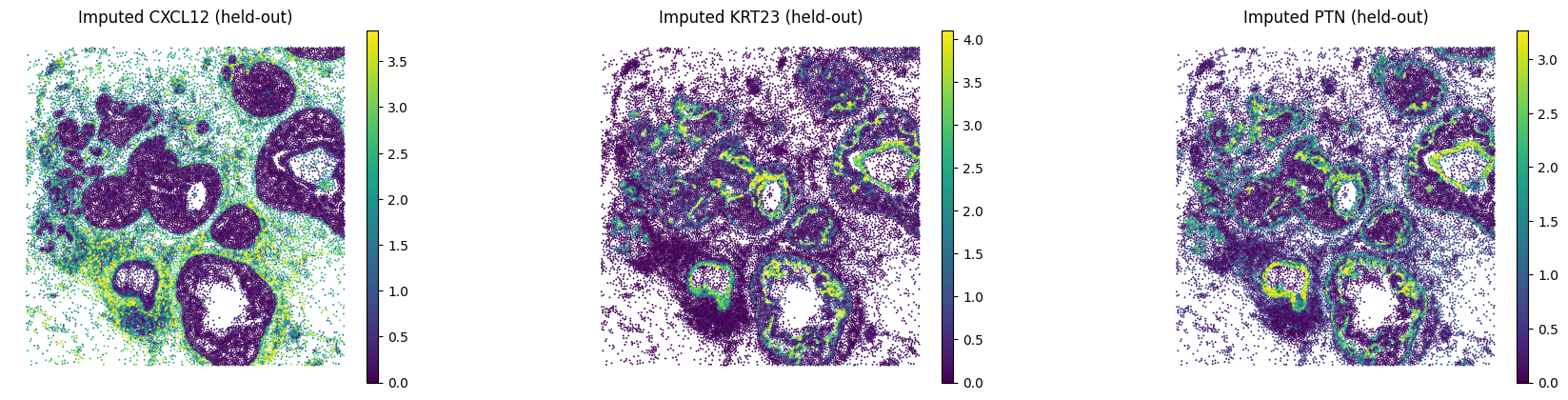
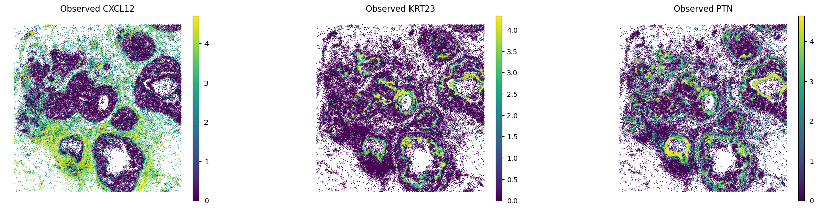
B.5 — Visualise held-out genes

Compare imputed vs. observed spatial expression for a few held-out genes with strong Pearson correlation.

# Edit: pick held-out genes with high Pearson from the evaluation above
GENES_HELDOUT = ["CXCL12", "KRT23", "PTN"]

sc.pl.spatial(
    adata_imputed_B,
    layer="imputed_norm",
    color=GENES_HELDOUT,
    spot_size=15,
    vmax="p99",
    frameon=False,
    title=[f"Imputed {g} (held-out)" for g in GENES_HELDOUT],
)
sc.pl.spatial(
    sp_adata,
    layer="log1p_norm",
    color=GENES_HELDOUT,
    spot_size=15,
    vmax="p99",
    frameon=False,
    title=[f"Observed {g}" for g in GENES_HELDOUT],
)